What is the leverage interest rate trading protocol RateX? How to effectively use RateX to maximize profits?
Written by: @seanhu001, Founder of RateX.

TLDR: This article covers three key areas
1. Understanding the Essence and Stability of JLP: The article introduces the principle of JLP and explains the reasons for its stable high returns.
2. Analyzing and Predicting JLP's APY: By breaking down the components of JLP APY (such as income sources and TVL), it helps readers understand the factors affecting APY and provides guidance for predicting short-term and long-term APY trends.
3. JLP Income Trading Strategies: The article introduces various trading strategies, including leveraged income speculation, fixed income investment, and APY-based arbitrage opportunities, providing practical insights for readers on income trading.
- Understanding the first leverage interest rate trading protocol RateX in the industry and how to effectively use RateX to maximize profits.
This year, JLP opportunities have been one of the most attention-grabbing asset types in the Solana ecosystem. Not only does it offer high returns, but it also maintains stable value, making it the preferred asset for many investors in the crypto bear market. This article will help readers understand the core of JLP and how to profit from analyzing and predicting JLP's APY.
1. What is JLP
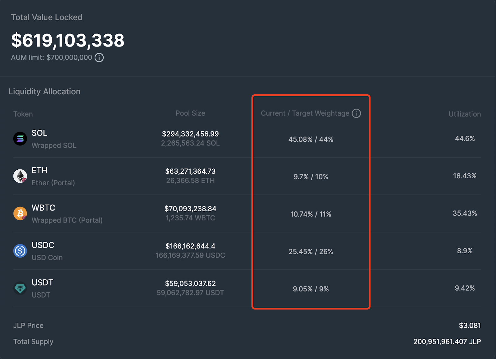
JLP is the liquidity pool of Jupiter Perp, consisting of assets such as SOL, WBTC, ETH, USDC, and USDT, with the latest composition ratio as follows.

The Target Weightage is set by the JUP team and adjusted by setting the Swap Fee or Mint/Redeem Fee. The Current Weightage represents the actual asset allocation in the pool. It can be seen that SOL has the highest proportion at 45%, with ETH and WBTC each accounting for nearly 10%. The remaining 25% and 9% are USDC and USDT, respectively.
How to understand the essence of JLP? Essentially, JLP is a combination loan pool of U-based and coin-based loans. We can divide the JLP Pool into two parts. The first part is the Crypto part, and the second part is the stablecoin part.
For the Crypto part, there are three assets, SOL, ETH, and BTC. The purpose of these assets is to lend to traders for long positions. Traders borrow these assets and repay the dollar value of the borrowed assets at the time. So, for every long crypto trade in the market, a portion of the value of crypto in the JLP becomes a dollar loan. When the utilization of a crypto asset such as SOL reaches 100%, we can understand that all SOL in the JLP has been converted into dollar loans.
For the stablecoin part, it supports two types of dollar-pegged stablecoins, USDC and USDT. The purpose of these assets is to lend to traders for short positions. Traders borrow these dollars and repay the amount of crypto in dollars borrowed at the time. So, for every short crypto trade in the market, a portion of the value of stablecoins in the JLP becomes a coin-based loan.
So we can simply get a formula to calculate the real stablecoin proportion of JLP:
Real stablecoin proportion = Real stablecoin quantity / TVL =

N represents the 3 assets in the crypto part, and m represents the 2 assets in the stablecoin part.
Through this formula, we can intuitively see that when the utilization of crypto assets is high (many long positions) and the utilization of stablecoin assets is low (few short positions), the value of JLP tends more towards a stablecoin pool. This means that in a bull market, with a large number of leveraged trades in the long direction, the value of JLP becomes more stable. Of course, JLP will experience a certain degree of impermanent loss (i.e., the value of the pool is lower than the value of its holdings in a bull market, but more stable).
Conversely, when the utilization of crypto assets is low (few long positions) and the utilization of stablecoin assets is high (many short positions), the value of JLP tends more towards a crypto pool. In other words, in a bear market, if long positions decrease and short positions increase, the value of JLP is more like a crypto combination.
However, in reality, it is not as we mentioned earlier. In the bear market, we can see that the long position ratio in Jupiter perp is still far greater than the short position. As of the time of writing this article (September 5th), the long/short ratio still reaches 90%.
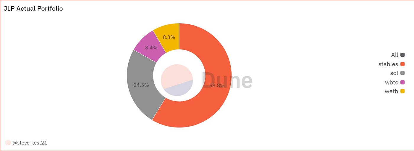
We can easily obtain the basic data of the current JLP Pool from here. According to our data analysis, the current real stablecoin proportion is 58.8%. This is also why we see the core reason for the value of JLP being so stable. When 60% of stablecoins are in the combination, its value is difficult to be unstable.

2. How to Predict JLP's APY
Let's look at another interesting point, the income data of JLP, which is reflected in their weekly APY data. Although JLP is an asset that accumulates income in the net asset value, its income is mixed with the fluctuation of the asset value in the pool. However, we can still analyze the income part from the value of JLP by using the official provided APY data or on-chain data.
Jupiter does not provide a historical time series of APY data, but we have created a 7-day average APY curve based on on-chain data. We can see that JLP's APY has consistently remained at a high income level, with significant fluctuations. With the gradual expansion of the JLP scale and the presence of a certain downward trend in the market, it still remains around 30%.

Next, we will analyze the composition of income in JLP and tell you how to predict the short-term and long-term trends of JLP's APY.
First, the calculation formula for JLP's APY is very simple:
APY = Earned Fees / TVL, and this section will mainly analyze and break down from the perspectives of earned fees and TVL.
1. Composition of Income Sources in JLP:
According to Jupiter's official documentation, we can see that the income sources of JLP mainly include the following factors:
The exchange generates fees and yields in various ways:
- Opening and Closing Fees of Positions (consisting of the flat and variable price impact fee).
- Borrowing Fees of Positions
Trading Fees of the Pool, for spot assets
Minting and burning of JLP
75% of the fees generated by JLP go into the pool.
Thanks to Jupiter, we can see the details of these income sources on-chain (related link)
These daily data form the basis for predicting JLP income.

We can see that pool_fees correspond to borrowing fees of the positions, swap_fees correspond to trading fees of the pool, oc_fees correspond to opening and closing fees of positions, and liq_fees should correspond to liquidation fees.

This chart reflects the time series data of Jupiter Perps Fees from July 23 to the present. We can see that oc_fees account for the absolute majority, so we mainly study oc_fees.
According to Jupiter's official website, the fee calculation for opening and closing positions involves the volume of these transactions, multiplied by the fee percentage of 0.06%. Of course, we know that this fee rate is dynamically adjusted by the official. Assuming the fee percentage remains unchanged, we know that oc_fees are linearly related to the trading volume. So as long as we can predict the trading volume, we can predict oc_fees.
We can obtain the trading volume of Jupiter Perps from on-chain data.

The following chart shows the trading volume on Solana's DEX.

We can see that the trading volume of Jupiter Perps and the trading volume on Solana's DEX have similar trends, but there is clearly greater independence. Despite a significant decrease in trading volume since July, the trading volume of Jupiter Perps has remained at a good level.
So when predicting short-term trading volume, we can accurately obtain Jupiter Perp's trading data through on-chain data analysis. However, when predicting the long-term trading volume trend, we need to consider both the trend of Solana's overall trading volume (beta) and the independent growth capability of Jupiter Perp as a proven successful project (alpha).
2. JLP's TVL Scale
After looking at the fee structure, let's take a look at TVL. This determines how much capital is available for leverage and also determines how many people are sharing the profits with you. From the chart below, we can see that JLP's TVL is steadily increasing. The Jupiter team's strategy for the growth of JLP's scale is relatively robust. They will set an AUM Limit for JLP to control the scale and prevent excessive TVL fluctuations from impacting LP income, which is a responsible approach in itself.

Overall, as the upper limit of JLP's TVL continues to increase, it is inevitable that the central APY will decrease. However, considering that we are currently in a bear market and the market trading volume has decreased by 50% since July, if the market heats up and Jupiter Perp's product itself remains competitive, we believe that JLP's APY is likely to rebound for a certain period of time, and it is not impossible to return to a level of 50%-60% APY or higher.
If you want to study short-term APY, for example, to obtain an expected JLP APY before the official announcement, you can visit the RateX official website. After the mainnet launch, click on JLP contracts in the market overview, and we will provide leading APY data for JLP for users to reference.
3. How to Profit from Predicting JLP's APY?
If you understand the research methods above and find predicting APY to be an interesting and simple task, then you need to read the following content, which will tell you how to make money through RateX's JLP yield trading feature.
- Speculate on future APY with leverage.
RateX is a leverage interest rate trading protocol that allows users to trade yield by creating synthetic YT-JLP. In simple terms, it creates a liquidity pool for JLP yield trading, where Liquidity Providers deposit JLP into this pool. Based on the deposited JLP, the protocol generates ST-JLP in the form of rebasing for Liquidity Providers.
The quantity of ST-JLP grows exponentially based on the official provided APY data, ensuring that the value of ST-JLP grows in line with the APY provided by JLP. At the same time, based on the deposited JLP, liquidity providers mint YT-JLP from the protocol (typically, depositing 1 JLP allows minting 1 YT-JLP).
Based on YT-JLP and ST-JLP, RateX has created a YT/ST AMM pool for users. When a trader wants to long YT with leverage, they deposit collateral (JLP) and the protocol creates ST-JLP for the user to buy YT-JLP in the AMM.
Conversely, if they want to short YT, they deposit collateral (JLP) and the protocol creates YT-JLP for the user to buy ST-JLP in the AMM.
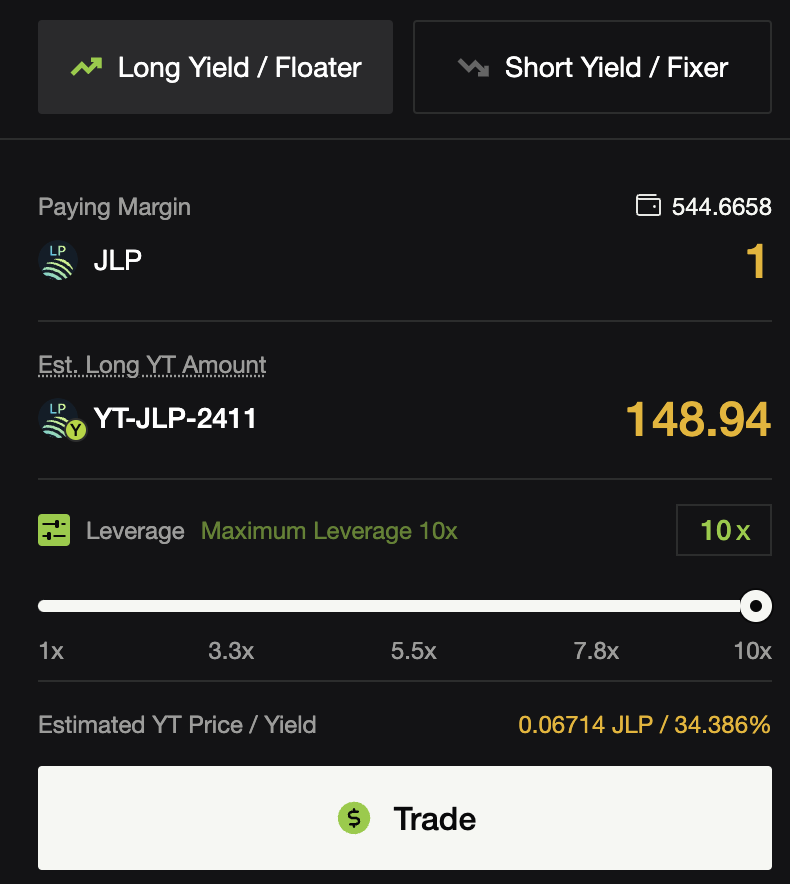
Currently, RateX can provide users with 10x leverage trading for YT-JLP.
In the JLP-2411 contract on the RateX testnet (expires at the end of November 24), depositing 1 JLP as collateral can buy 148.94 YT-JLP-2411.

Since the price of YT follows the following formula:

This is a non-linear formula, which may not be intuitive. When the implied yield is smaller, you can roughly assume that the rate of change in the YT price is the same as the percentage change in the Implied Yield (APY). (For example, for a contract expiring in six months, when the implied yield changes from 3% to 4%, the YT price change is roughly 4%/3%-1=33%. When it changes from 30% to 40%, the YT price change percentage is roughly 26%. There is a sensitivity issue with the discount factor here). If you are a mature investor, we still recommend that you calculate it yourself for more accuracy. There is a detailed explanation for YT here.
2. Fixed Income Investment
RateX constructs PT assets based on YT and ST, where PT=1-YT. Because YT is an asset whose value tends to zero as it continues to receive yield, the value of PT will gradually approach that of ST-JLP. If you choose to hold until maturity, you will receive a fixed income, which is a conservative passive income strategy in itself.
You can also choose to implement a PT spread strategy. If the YT price falls (implied yield decreases), the PT price will rise, and you can choose to redeem PT immediately to obtain a higher annualized return.
You can also choose a strategy similar to Kamino multiply, where you collateralize PT to borrow funds to continue buying PT, generating higher returns. Of course, after adding leverage, you need to be careful of liquidation risks.
3. Arbitrage Trading
There is also a strategy based on predicting the APY of the YT interest payment cycle for arbitrage trading. Since YT is a time-decaying asset, its value is amortized based on the implied yield. We will revalue the YT at the end of each interest payment cycle. If the decrease in value does not match the value of the yield received, you have the opportunity to arbitrage by predicting the APY data. For example, if you buy a YT at a 30% implied yield, and in the next interest payment cycle, the implied yield is still at 30%, but you receive a yield of 50%, and the value of your YT has decreased based on the 30% implied yield as time passes. This means that you have received more yield than the decrease in the value of YT. If you can immediately sell the YT at the market price, you have the opportunity to arbitrage by predicting the APY within this interest payment interval. However, this short-term arbitrage opportunity is very small, and the implied yield of YT reflects the expected average APY over the remaining term. Therefore, failing to arbitrage during the interest payment cycle may become a source of profit for longer-term strategy traders. Therefore, unless you are a professional trader, it is not recommended to participate.
After reading this article, if you find it helpful, you can follow our Twitter account: @RateX_Dex to learn more about income trading opportunities.
免责声明:本文章仅代表作者个人观点,不代表本平台的立场和观点。本文章仅供信息分享,不构成对任何人的任何投资建议。用户与作者之间的任何争议,与本平台无关。如网页中刊载的文章或图片涉及侵权,请提供相关的权利证明和身份证明发送邮件到support@aicoin.com,本平台相关工作人员将会进行核查。


